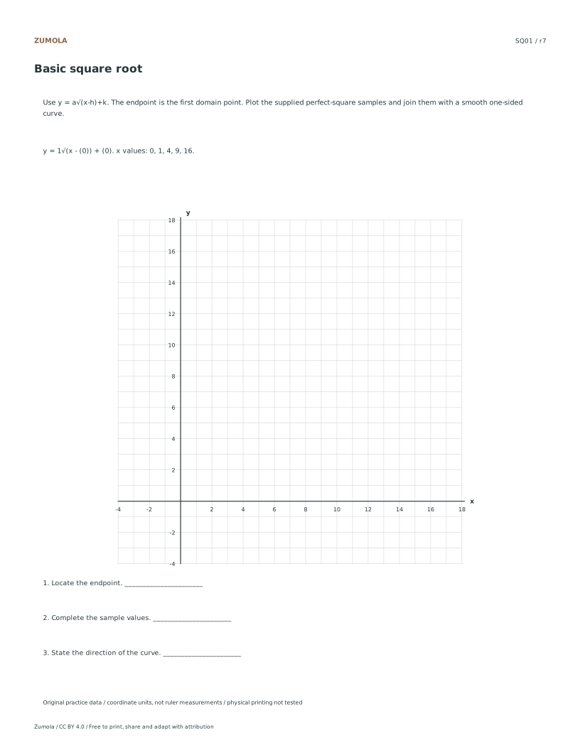
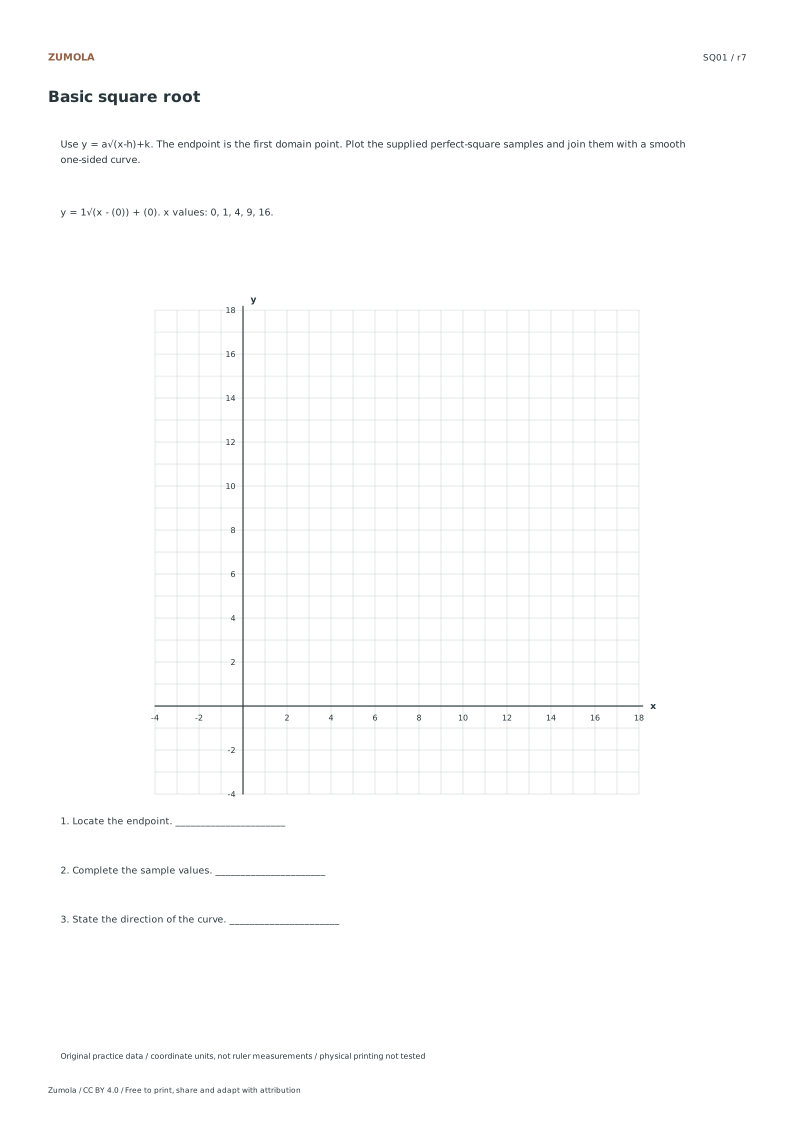
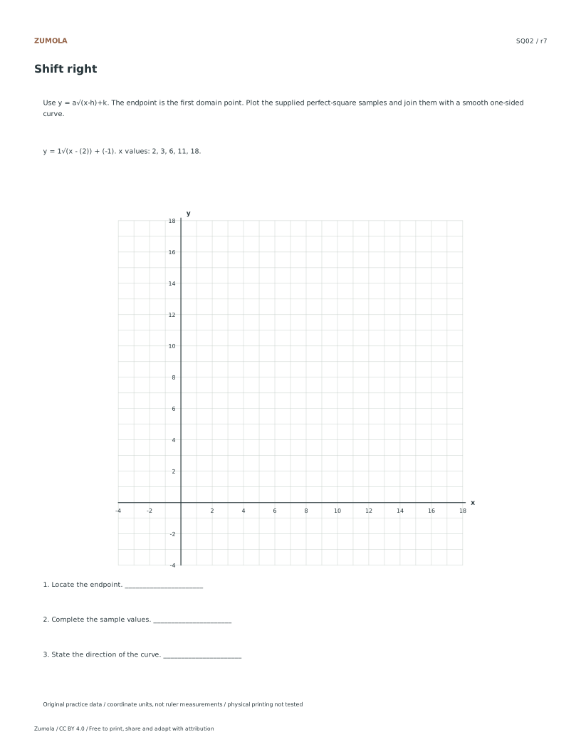
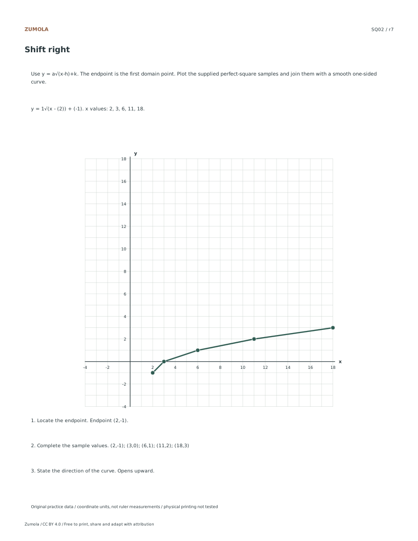
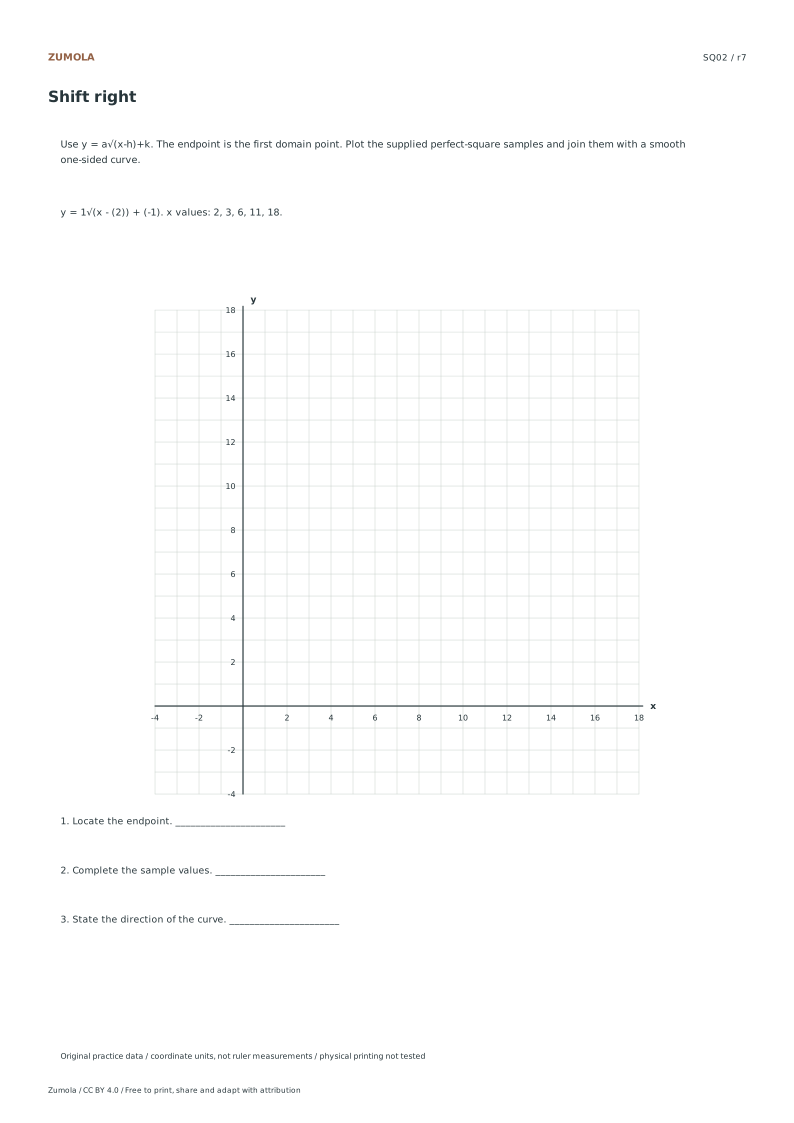
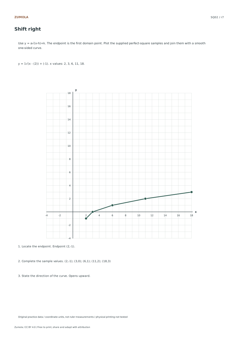
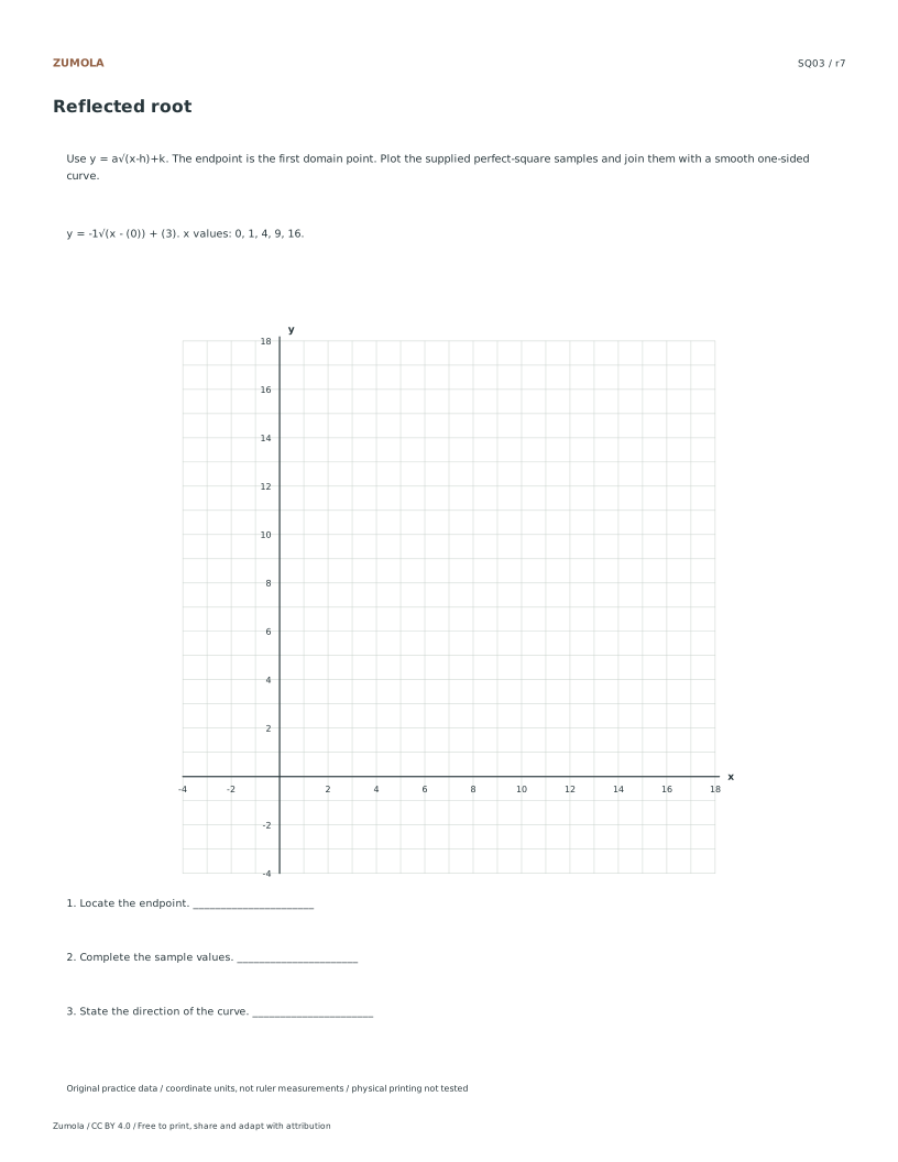
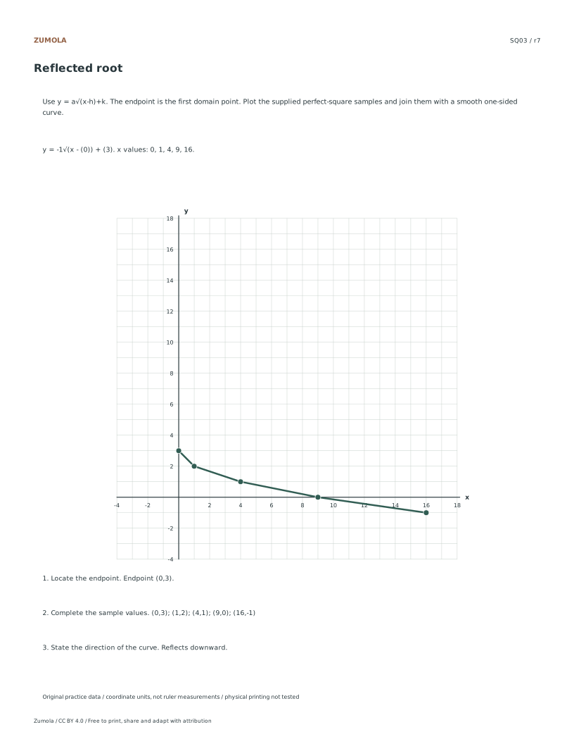
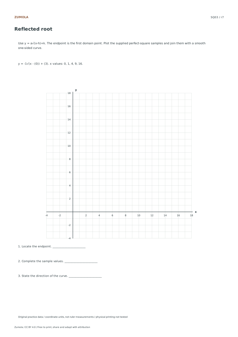
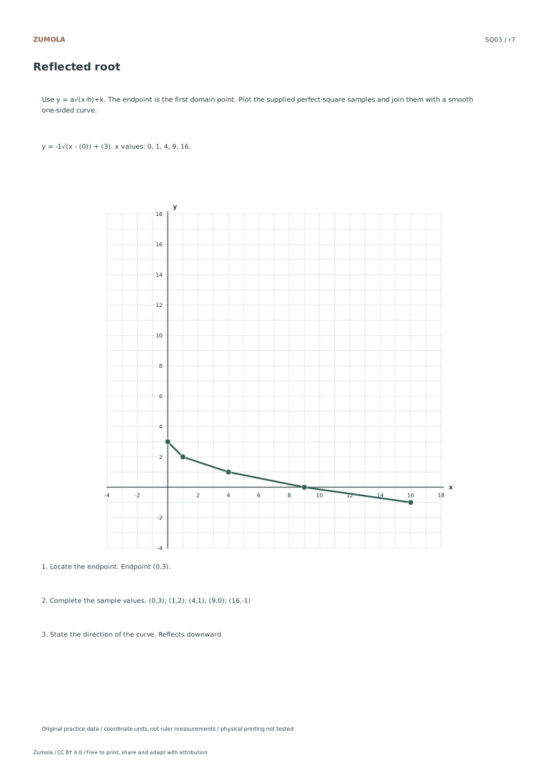
Plot four one-sided radical curves from y=a√(x-h)+k. Locate the endpoint, complete perfect-square samples and compare reflected and shifted roots.
Choose Letter or A4, then download a student sheet first. Keep the separate reference or answer file closed until you have attempted the case. Every worksheet, SVG and answer is free without signup.
Choose your paper and download
Download paper size
Every worksheet and answer is free. No signup.
Free original resourceSQ01
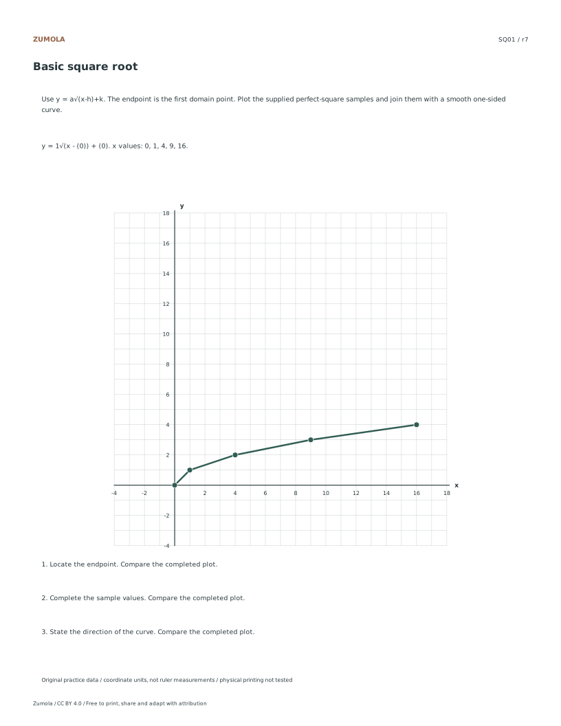
Basic square root
Original worksheet collection. Letter or A4 PDF and editable SVG.
All examples use original fictional data and coordinate units. They are practice material, not measured classroom results, published questions or evidence about real people.
Check the first case
SQ01: Basic square root
Check
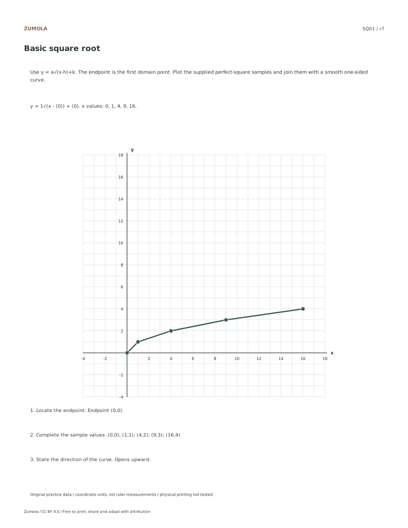
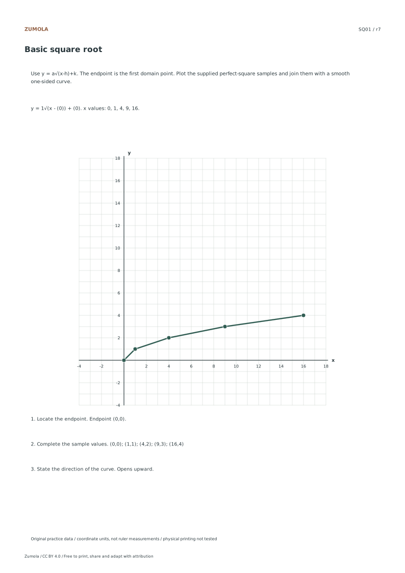
Worked result
1
Endpoint (0,0).
2
(0,0); (1,1); (4,2); (9,3); (16,4)
3
Opens upward.
The first case shows the checking pattern. Individual answer files contain the completed graph and result for every case.
Work through the graph
Identify the Starting Point
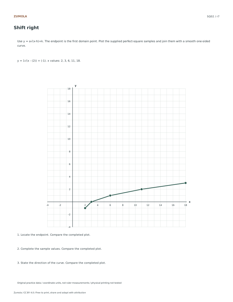
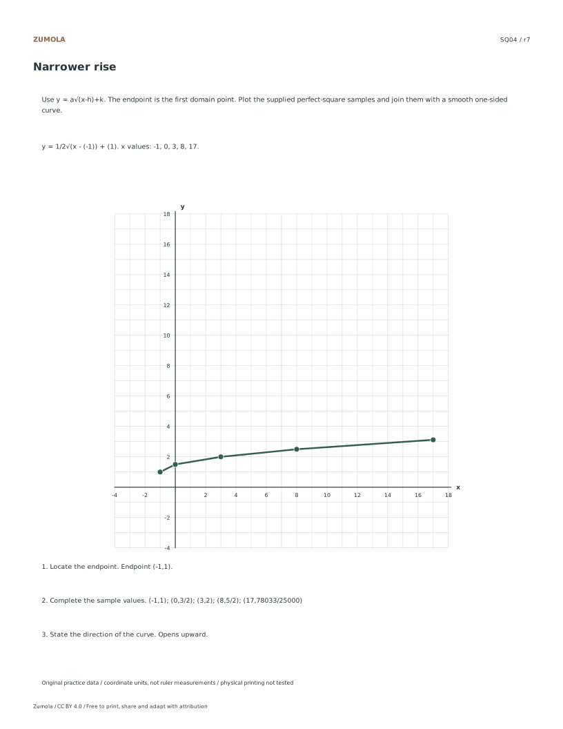
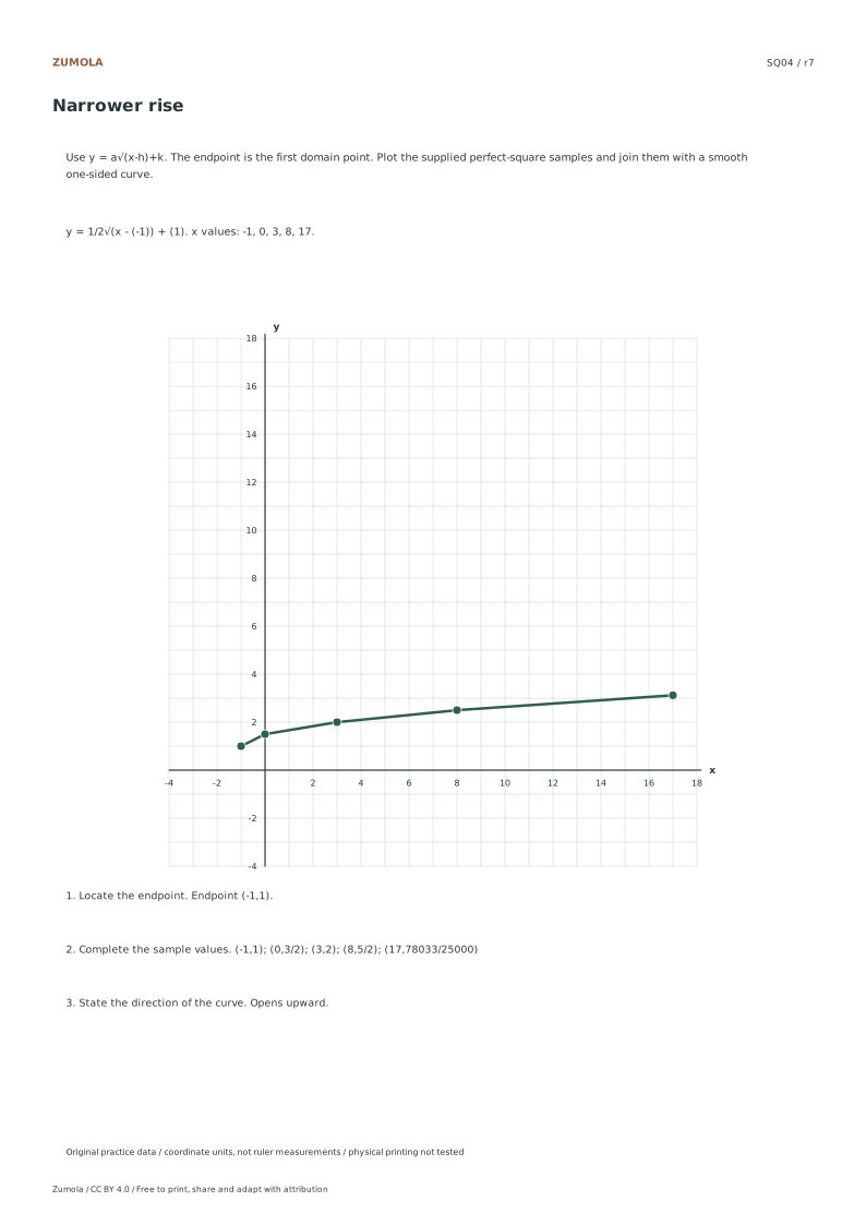
Begin by locating the endpoint of the curve using the horizontal shift value h. This coordinate marks the leftmost point of the graph because the domain begins at h. For example, in the shift right case, the endpoint is at x equals two. Mark this point clearly on your grid before plotting other values. This step ensures the curve starts in the correct position. The vertical shift k determines the y coordinate of this endpoint. Combining h and k gives the precise starting location. This foundational step prevents misalignment when connecting subsequent points. It establishes the anchor for the entire function shape. Ensure you distinguish this from the y intercept if it exists. The endpoint is always the first value in the domain range.
Plot Sample Coordinates
Use the provided table of x values to calculate corresponding y coordinates. These x values are chosen so that horizontal offsets from h are perfect squares. This simplifies the square root calculation significantly. For instance, if h is zero, x values like one, four, and nine yield integer results. Substitute each x into the function formula to find y. Plot these points accurately on the coordinate plane. Do not connect them with straight lines yet. Each point represents a specific solution derived from listed coordinates. The supplied values determine these answers exactly. Verify that the offset from h is indeed a perfect square. This ensures the arithmetic remains manageable and precise. Plotting these points creates the skeleton of the curve.
Draw the Smooth Curve
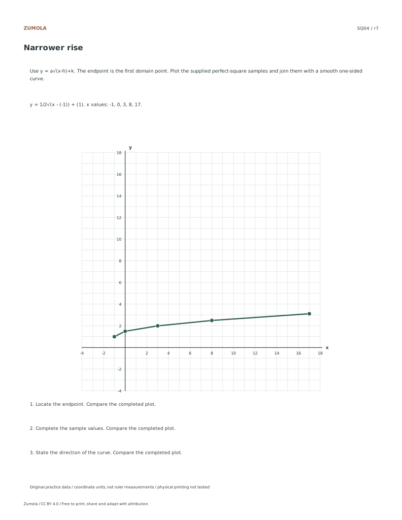
Connect the plotted points using a smooth one-sided curve. Start at the endpoint and extend through the sample points. The curve should not have sharp corners or breaks. If the coefficient a is negative, the curve reflects vertically. This means it opens downward instead of upward. For the narrower rise case, the curve rises more steeply. Ensure the line passes through all calculated points. Do not extend the curve to the left of the endpoint. The domain restriction means the graph exists only for x greater than or equal to h. Use a steady hand to maintain smoothness. This visual representation completes the graphical solution. Check that the shape matches the function type. The curve should look natural and continuous.
Checks that catch common errors
Watch for
Check instead
Extending the curve to the left of the endpoint
The domain begins at h, so the graph exists only for x values greater than or equal to h. Stop the curve at the endpoint and do not draw any line to the left of this point. The one-sided nature is a key feature of square root functions.
Connecting points with straight line segments
Square root functions produce curved graphs, not linear ones. Use a smooth curve to connect the plotted points. Straight lines between points create a jagged appearance that misrepresents the function. Ensure the transition between points is gradual and continuous.
Ignoring the vertical reflection when a is negative
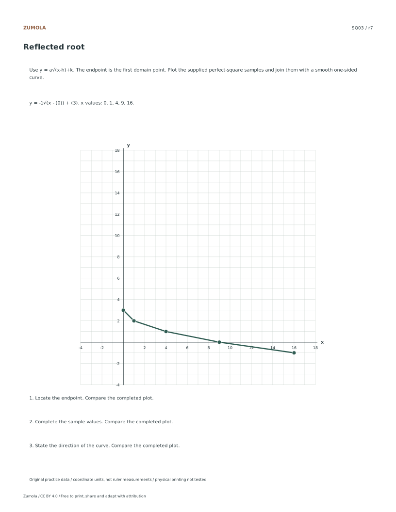
A negative coefficient reflects the curve vertically across the horizontal axis. If a is negative, the curve opens downward from the endpoint. Check the sign of a before drawing. For the reflected root case, the curve decreases as x increases.
Keep the labels and margins readable
Choose the PDF that matches your paper. Print at Actual size / 100% and turn off Fit, Shrink and browser headers. SVG is editable but an editor can rescale it; the PDF is the simpler print route. Physical printer, classroom and curriculum tests have not been completed.
Useful answers
Where does a square-root graph begin?
At x=h in y=a√(x-h)+k, the endpoint is (h,k).
Why are the sample x values uneven?
They make x-h perfect squares, which makes the sample values easy to check.
What does a negative a do?
It reflects the curve vertically, so it travels downward from the endpoint.
Are the answer files and editable graphs free?
Yes. The individual student, reference and answer files plus collection packs are free without signup. Credit Zumola under CC BY 4.0 when sharing or adapting.
Further reading: OpenStax: radical functions. The diagrams, datasets and exercises here are original Zumola work.
Your analytics choice
Optional Google Analytics helps us understand which free resources are useful. It is off until you allow it. Drawing tools and downloads work with either choice. Privacy details